1. Origin and Background of BrainFlow

BrainFlow is an open-source biosensing data acquisition SDK created by Andrey Parfenov in 2018. Parfenov – a software engineer with experience at Intel, Nvidia, and research at the University of Innsbruck – started BrainFlow as a personal project after finding the official OpenBCI Python SDK difficult to use. Initially, there was no company or grant behind BrainFlow; it was born out of the need for a more robust, uniform way to programmatically access devices like the OpenBCI Cyton board.

Evolution: BrainFlow began as a replacement for the OpenBCI Hub (a middleware used by older OpenBCI GUIs) and quickly evolved into a full-fledged cross-platform SDK. By 2020, OpenBCI officially adopted BrainFlow in their GUI v5.0 as the primary data acquisition library, eliminating the old “Hub” process. This integration highlighted BrainFlow’s reliability and performance improvements. The project has since grown with contributions from the community and support via OpenBCI (Andrey Parfenov became an OpenBCI team member). BrainFlow remains open-source (MIT-licensed) with funding through its Open Collective and support from companies like OpenBCI.

Affiliations and Contributors: BrainFlow is not tied to a single institution; it’s a community-driven project led by Parfenov. OpenBCI is a major partner – providing long-term support funding and integrating BrainFlow into their software ecosystem. Over the years, BrainFlow’s contributor base expanded (1000+ Slack members and dozens of contributors by 2023)brainflow.org. The project emphasizes good software engineering practices (CI tests, device emulators, strict code reviews) to maintain reliability across its broad scope. In summary, BrainFlow’s origin lies in one developer’s initiative to improve neurotech tooling, and it has grown into a widely-used SDK underpinning many BCI applications (including the official OpenBCI GUI).

2. Setting up BrainFlow in a Conda Environment on macOS M3

Setting up BrainFlow on an Apple Silicon Mac (M1/M2/M3) using Conda is straightforward. The key is to use an ARM64 Conda distribution (such as Miniforge/Mambaforge) and then install BrainFlow via pip. Below are step-by-step instructions, along with tips for serial port configuration and troubleshooting on Apple Silicon Macs:

• Step 1: Install an ARM64 Conda – On an Apple M3 (Apple Silicon) Mac, install Miniforge or a similar Conda that supports arm64. This ensures all packages (including Python) are optimized for Apple Silicon.

• Step 2: Create a new environment – It’s recommended to use Python 3.9+ (BrainFlow supports Python 3.x; version 3.10 or 3.11 works well). For example:

conda create -n brainflow-env python=3.10 numpy matplotlib pyqt  # create env with common packages
conda activate brainflow-env

• Step 3: Install BrainFlow via pip – BrainFlow is not on the main Conda channels, so use pip inside the environment:

pip install brainflow

pip install pyserial

pip install pyqtgraph pyqt5

This downloads a prebuilt Python wheel with universal binaries for macOS (since BrainFlow 4.3.1, the pip package includes both x8664 and arm64 libraries) brainflow.org. Make sure the pip output indicates an arm64 or universal install to avoid architecture mismatches (the _mach-o wrong architecture error was resolved by the universal build) brainflow.org.

• Step 4: Connect the OpenBCI dongle – The Cyton board uses an FTDI USB serial dongle. On macOS, no separate driver installation is needed for Apple Silicon; macOS’s built-in FTDI driver will handle it. (FTDI’s official drivers are x86_64-only and will not load on ARM Macsopenbci.com.) When you plug in the dongle, macOS will create two device nodes: /dev/tty.usbserial-D#### and /dev/cu.usbserial-D####. Always use the /dev/cu.* port with BrainFlow (the tty form can block or wait for a modem signal).

• Step 5: Set up serial port permissions – Typically, on macOS, your user should have access to /dev/cu.usbserial*. If you encounter permissions errors, you may need to adjust by adding your user to the dialout/tty group or running with sudo (though macOS usually doesn’t require this for USB serial devices). Ensure the Conda environment has permission to access the serial port (if running Jupyter, you might need to grant the Terminal “Full Disk Access” in macOS Privacy settings for it to see serial devices).

• Step 6: Verify BrainFlow can detect the board – You can run a quick Python test in the conda environment:

conda install -n brainflow-env ipykernel --update-deps --force-reinstall

from brainflow.board_shim import BoardShim, BrainFlowInputParams, BoardIds  
params = BrainFlowInputParams()  
params.serial_port = "/dev/cu.usbserial-DXXXX"  # put your port here  
board = BoardShim(BoardIds.CYTON_BOARD.value, params)  
board.prepare_session()  
print("Session prepared, board info:", BoardShim.get_board_descr(BoardIds.CYTON_BOARD.value))  
board.release_session()

This should initialize communication with the Cyton dongle. If there’s an error like “unable to open port”, double-check the port name and that no other program (e.g., the OpenBCI GUI) is using the dongle.

• Handling FTDI Latency on Apple Silicon: A known issue on macOS 11+ with Apple M1/M2/M3 is the FTDI latency timer defaulting to 16 ms, which can cause choppy data or timestamp jitter. In other words, the dongle’s USB driver buffers data ~16ms before delivering, leading to a slight lag and uneven packet timing. On Intel Macs this could be adjusted via a driver setting, but on Apple Silicon the built-in driver doesn’t allow easy configuration via .plist. As a workaround, you can use a small utility to set the latency to 1 ms at runtime. For example, installing libftdi1 (via Homebrew) and running a C program to adjust latency each time the dongle connects has been shown to fix the stutter. This step is optional – even with the 16 ms buffer, data will still be delivered correctly at 250 Hz, just with a constant small delay. If ultra-low latency is crucial (e.g., for neurofeedback), consider the libFTDI tweak or use the OpenBCI WiFi shield (which streams data over network rather than serial).

• USB-C Adapter Note: If using a Mac that only has USB-C ports, use a reliable USB-C to USB-A adapter for the OpenBCI dongle. Some cheap adapters can introduce their own latency or throughput issues. If you notice unusually slow data or connection issues, try a different adapter.

By following the above steps, you’ll have BrainFlow installed in a Conda environment on your Apple Silicon Mac. Python 3.10+ is recommended for best compatibility (as many scientific libraries and BrainFlow itself fully support Python 3.10+). The Conda environment isolates the dependencies, and using pip inside Conda is fine in this case (BrainFlow’s Python wheel includes the necessary native libraries).

Troubleshooting Tips: If you get a library load error, ensure that your Python itself is running natively (arm64). Running an x86_64 Python under Rosetta can cause mismatch with BrainFlow’s arm64 libs. Conda-forge’s Python will be arm64 on M1/M2/M3, but double-check by running uname -m in Python (platform.machine()) – it should return arm64. Also, if you previously installed an FTDI driver, you might need to remove it to let the Apple driver take over (FTDI’s installer might place a kext that is not arm64-compatible, as seen in error logsopenbci.com). Removing or updating that can resolve port access issues.

3. Using BrainFlow with OpenBCI Cyton (8-Channel EEG)

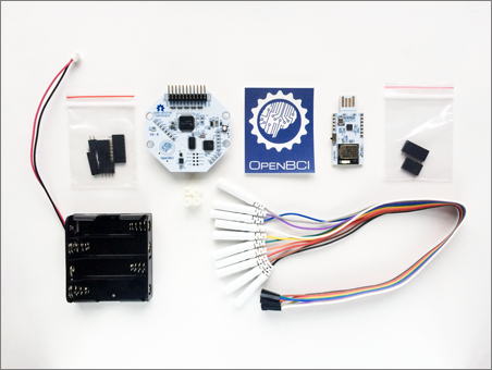
The OpenBCI Cyton is an 8-channel EEG board, and BrainFlow has first-class support for it. Here we focus on connecting a Cyton (with its USB dongle) on macOS, what data BrainFlow returns, how the 8 channels are organized, and any gotchas on Apple Silicon Macs.

Connecting to Cyton on macOS: The Cyton communicates via an RFduino USB dongle, which creates a serial port. After plugging in the dongle, find the port name (on macOS it will be something like /dev/cu.usbserial-D123 as mentioned). In your BrainFlow code, you’ll specify:

• Board ID: use BoardIds.CYTON_BOARD (or value 0 – but the enum is clearer).

• Serial port: set BrainFlowInputParams().serial_port to the /dev/cu.usbserial-XXXX path.

No other parameters are needed for basic operation. For example, in Python:

from brainflow.board_shim import BoardShim, BrainFlowInputParams, BoardIds
params = BrainFlowInputParams()
params.serial_port = "/dev/cu.usbserial-D123"  # replace with your port
board = BoardShim(BoardIds.CYTON_BOARD.value, params)
board.prepare_session()
board.start_stream()
# ... (data acquisition loop)
board.stop_stream()
board.release_session()

That’s all it takes to start getting data. Under the hood, BrainFlow knows the Cyton’s baud rate, packet format, number of channels, etc. If the dongle is properly paired with the Cyton (it comes pre-paired from the factory, indicated by the LED status), board.start_stream() will begin transmitting EEG packets. By default, Cyton samples at 250 Hz per channel (8 channels), so you’ll get data at that rate. You can optionally change the sample rate (Cyton firmware supports 125 Hz or 250 Hz) by sending a config string via board.config_board("<command>") – but 250 Hz is the default and typical setting.

Data returned (EEG, AUX, timestamps, markers): When you call board.get_board_data(), BrainFlow returns a 2D array of shape (N_channels x N_samples). The Cyton board in default mode sends 8 EEG channels plus 3-axis accelerometer and one other analog channel, plus timestamp. BrainFlow’s channel ordering for Cyton is typically:

• Channels 0–7: EEG data from the 8 electrodes (in microvolts). These correspond to the Cyton’s analog inputs D0–D7. If you’re using the standard OpenBCI headcap or electrode placements, you might label them according to 10-20 locations (for example, an Ultracortex Mark IV with 8 nodes often uses locations like Fp1, Fp2, C3, C4, P7, P8, O1, O2 – but this mapping is user-defined, not inherent to Cyton) pypi.org. BrainFlow doesn’t assign channel names, but you can map them as needed. You can retrieve the indices via BoardShim.get_eeg_channels(BoardIds.CYTON_BOARD) which would return [0,1,2,3,4,5,6,7] (for Cyton’s EEG channels).

• Channels 8–10: Aux data, which on Cyton is the onboard accelerometer X, Y, Z axes (in g or raw units). If you don’t need motion data, you can ignore these. (Note: The Cyton’s accelerometer data comes at the same 250 Hz rate, but it’s 8-bit values interleaved in the radio packet – BrainFlow extracts and scales them).

• Channel 11: Cyton has an analog channel for battery or other inputs (on some firmware this might carry battery voltage or other ADC channel). This might appear as well (some BrainFlow docs indicate Cyton has 8 EXG + 3 accel + 1 analog = 12 data channels plus timestamp).

• Last channel: Timestamp – BrainFlow always appends a timestamp for each sample, and often a marker channel as well. In many cases, BrainFlow’s output array includes a dedicated timestamp column (in UNIX time or milliseconds) and a marker column (initialized to 0). You can get the index with BoardShim.get_timestamp_channel(board_id) and BoardShim.get_marker_channel(board_id). For Cyton, the timestamp channel index is typically the last one (since Cyton’s own data has no timestamp, BrainFlow injects it when the packet is received). The marker channel, if present, might be last or second-last depending on implementation.

In practice, a safe way to parse the data is: use BrainFlow’s API calls to get channel indices for each type. For example:

eeg_indices = BoardShim.get_eeg_channels(BoardIds.CYTON_BOARD.value)
acc_indices = BoardShim.get_accel_channels(BoardIds.CYTON_BOARD.value)
marker_index = BoardShim.get_marker_channel(BoardIds.CYTON_BOARD.value)
timestamp_index = BoardShim.get_timestamp_channel(BoardIds.CYTON_BOARD.value)
data = board.get_board_data()
eeg_data = data[eeg_indices, :]    # numpy slice of EEG
timestamps = data[timestamp_index, :]

The 8-channel EEG layout doesn’t inherently correspond to specific scalp locations until you set up the hardware. Each channel is just a voltage measurement from the EXG amplifier. When you plug in an electrode at, say, input 1 and place it on Fp1 on the scalp, then channel 1 corresponds to Fp1. So interpretation is up to your montage. OpenBCI’s documentation provides guidance on mapping the Cyton’s inputs to 10-20 positions if using their headset (as shown above in the BrainflowCyton example list)pypi.org. By default, channel numbering in software is 0–7, but the OpenBCI GUI labels them 1–8 for user-friendliness.

Markers on Cyton: If you insert markers via board.insert_marker(val), BrainFlow will inject the val into the marker channel of the next data samplebrainflow.readthedocs.io. On Cyton, there is a limitation: the RFduino radio protocol transmits 3 auxiliary bytes per sample (used for accelerometer by default). To accommodate a custom marker value, BrainFlow’s Cyton implementation repurposes those bytes for the marker. This means when you use marker functionality, the accelerometer readings will be overwritten or disabled while the marker is setpypi.org. In other words, Cyton cannot send both a custom marker and accelerometer simultaneously in one sample – BrainFlow chooses markers over accel for those packets. This is usually fine (you typically don’t need continuous accel if you’re inserting event markers), but it’s good to be aware. The marker channel itself will appear in the data array (often all zeros except at the moments you inserted a value). For example, if you call insert_marker(1.0) at some time, you’ll later see a “1.0” in the marker channel array at the corresponding index, which you can use to tag events.

Known limitations / bugs on Apple Silicon: Aside from the FTDI latency issue discussed (which causes slight jitter but no data loss), the Cyton + BrainFlow generally works very reliably on M1/M2/M3 Macs. The most common “gotcha” is making sure to use the correct serial port. Also, if you put the Mac to sleep or unplug the dongle, you should release_session() and handle reconnects properly – occasionally the serial port might not close cleanly if an app is force-quit, requiring you to replug the dongle. Another edge case: Some USB-C hubs might cause slow data (if they internally introduce a USB 1.1 bottleneck), so if you see a throughput issue, test different ports/hubs.

BrainFlow’s Cyton support includes advanced features like analog “Analog” and **Digital modes as well (Cyton can switch to send 4 AUX analog inputs instead of EEG, etc.), which can be activated via config_board commands if needed. For instance, Cyton has an “Analog mode” where instead of accelerometer, it sends additional analog readings – BrainFlow 2.0 added support for Cyton’s analog modebrainflow.org. These are more specialized use cases (for reading external sensors on Cyton’s AUX pins). For most users, the default EEG mode is ideal.

In summary, BrainFlow treats the Cyton’s 8-channel EEG stream as just another board – you get a block of raw EEG data in microvolts, along with timestamps and any aux data, at 250 Hz. The 8 channels correspond to whatever electrodes you’ve connected; BrainFlow doesn’t assume specific positions. It’s up to you to know that, for example, Channel 0 = “Fp1” if that’s how you set up your cap. The data can then be filtered, visualized, or analyzed using BrainFlow’s processing functions or exported to other libraries (like MNE or EEG.io). The integration is seamless on macOS M3 – BrainFlow abstracts away all the Bluetooth pairing or serial port peculiarities, leaving you with a clean Python (or Java/C++) interface to the Cyton.

4. Jupyter Notebook Template – BrainFlow + OpenBCI Cyton Example

Finally, let’s put everything together with an example Jupyter Notebook workflow. This example will demonstrate how to:

• Initialize a BrainFlow session for the Cyton board.

• Start the stream and read real-time EEG from the 8 channels.

• Plot the live data using pyqtgraph (which is well-suited for real-time plotting in notebooks or GUIs).

• Insert event markers (as an example, we’ll add a marker every few seconds).

• Save the data to a file for later analysis.

Prerequisites: In your Conda environment, ensure you have brainflow installed (as above) and also install pyqtgraph. You might also need to install PyQt5 for pyqtgraph to use (on macOS, using pip install pyqt5 or brew install pyqt@5 and setting up the Qt backend if in Jupyter). Matplotlib is optional here, but we will use pyqtgraph for live plotting due to its performance.

Here’s a step-by-step Notebook script (with commentary inline):

# Import necessary packages
import numpy as np
import pyqtgraph as pg
from pyqtgraph.Qt import QtCore, QtWidgets
from brainflow.board_shim import BoardShim, BrainFlowInputParams, BoardIds

# 1. Configure BrainFlow for Cyton board
BoardShim.enable_dev_board_logger()  # Optional: enable logging for debug
params = BrainFlowInputParams()
params.serial_port = "/dev/cu.usbserial-D123"  # <-- put your Cyton dongle port here
board = BoardShim(BoardIds.CYTON_BOARD.value, params)

# 2. Prepare and start the BrainFlow session
board.prepare_session()               # Initialize connection
board.start_stream() # Start streaming (buffer holds 45000 samples ~ 180s at 250Hz)
print("BrainFlow streaming started...")

# 3. Set up live plotting with pyqtgraph
app = QtWidgets.QApplication([])
win = pg.GraphicsLayoutWidget(show=True, title="OpenBCI Cyton EEG Stream")
plot = win.addPlot(title="Real-time EEG")
plot.showGrid(x=True, y=True)
plot.addLegend()
plot.setRange(yRange=[-100, 100])  # µV range for EEG
curves = []
for ch in range(8):
    curve = plot.plot(pen=pg.intColor(ch, hues=8), name=f"Ch{ch+1}")
    curves.append(curve)

# 4. Define an update function to pull data and update the plot
def update():
    # Get latest data (without removing from buffer):
    data = board.get_current_board_data(num_samples=1250)  # get 1 second of data (250 samples)
    if data.shape[1] > 0:
        eeg_channels = BoardShim.get_eeg_channels(BoardIds.CYTON_BOARD.value)
        sampling_rate = BoardShim.get_sampling_rate(BoardIds.CYTON_BOARD.value)
        for ch in eeg_channels:
	        DataFilter.perform_bandpass(data[ch], sampling_rate, 1.0, 50.0, 4, FilterTypes.BUTTERWORTH.value, 0)
	        DataFilter.perform_bandstop(data[ch], sampling_rate, 48.0, 52.0, 2,FilterTypes.BUTTERWORTH.value, 0)
		offset = 150
        # For each EEG channel, update its curve with new data
        for idx, ch in enumerate(eeg_channels):
            # We will plot the last N samples from that channel
            y = data[ch] + (idx * offset)  # EEG values in µV
            x = np.arange(len(y))
            curves[idx].setData(x, y)
        # (Note: This plots each channel's waveform overlapping; for clarity, one might offset them or use a scrolling X axis.)

# 5. Use a QTimer to call the update function periodically (20 Hz refresh)
timer = QtCore.QTimer()
timer.timeout.connect(update)
timer.start(50)  # 50 ms interval -> ~20 updates per second

# 6. (Optional) Insert event markers in the stream
marker_interval = 5  # seconds
def insert_marker():
    board.insert_marker(1.0)  # insert a marker value of 1.0
    QtCore.QTimer.singleShot(marker_interval * 1000, insert_marker)
# Schedule the first marker insertion
QtCore.QTimer.singleShot(marker_interval * 1000, insert_marker)

# 7. Start the Qt event loop to show the plot window and begin updates
QtWidgets.QApplication.instance().exec_()

# 8. When done, stop stream and release session
board.stop_stream()
board.release_session()
print("Session stopped and released.")

Let’s break down what this notebook code is doing:

• We create a BoardShim for the Cyton and start the stream. We specified a large buffer (45000 samples) for BrainFlow internally – this doesn’t affect real-time operation but ensures we can retrieve up to 3 minutes of data if needed. (In practice, we use get_current_board_data for the latest chunk.)

• We set up a pyqtgraph plotting window with 8 curves, one for each EEG channel. The Y-range is set to ±100 µV for visibility (you can adjust depending on signal amplitude). Each channel gets a different colored pen.

• The update() function pulls the latest ~250 samples (1 second) of data from BrainFlow’s internal ringbuffer without clearing it (get_current_board_data gives current data whereas get_board_data clears the buffer). It then updates each curve’s data. This will make the plot display a moving waveform for each channel. In this simple example, we’re plotting each channel on the same axes (overlapping). For a multi-channel chart, you might instead stack them or use offsets, but overlapping gives an EEG trace view.

• A QTimer is set to call update() every 50 ms (20 Hz refresh rate), which is smooth enough for visualizing 250 Hz data.

• We also demonstrate inserting an event marker: using another timer (singleShot) to call board.insert_marker(1.0) every 5 seconds. This will inject a “1” in the marker channel periodically. (In a real experiment, you’d call insert_marker at specific event times, e.g., when a stimulus is presented. Here we simulate an event every 5 seconds.)

• Finally, we start the Qt event loop with app.exec_(). This line is what hands control to the GUI so the window stays open and updates. In a Jupyter Notebook, you might need to run the cell in a different async manner or use %gui qt magic to integrate Qt’s loop – depending on your Jupyter environment, the specifics vary. Another approach in Jupyter is to not use Qt at all but rather gather data and use matplotlib’s animation functions; however, real-time interactivity is better with pyqtgraph as shown.

• After you close the plot window (or interrupt the loop), the code stops the stream and releases the board session, which is important to free the dongle for future use.

Running this notebook: When you run the above code in a Jupyter environment on macOS, a window should pop up showing rolling EEG traces from the Cyton in real time. You’d see 8 traces updating. (If running on a headless server, you won’t have a display for Qt – in that case, consider using matplotlib inline plots of chunks instead, but on a local Mac you should be able to open windows.)

You can also log data to a file simultaneously. One easy way is to use BrainFlow’s streamer: for example, instead of board.start_stream() you could do board.start_stream(45000, "file://eeg_data.csv:w") which would write all incoming data to eeg_data.csv in write mode. The rest of your code can still fetch and plot data. This built-in logging is very handy for keeping a record. Alternatively, you could collect data in a list and use pandas to save to CSV at the end (BrainFlow’s own CSV format matches what OpenBCI GUI outputs, with columns like EEG channels, Accel, etc., and a header in the file).

Inserting markers and interpreting them: In the above code, we insert a marker of value 1.0 every 5 seconds. If you open the saved CSV, you won’t directly see the marker in the main columns, because the marker is in its own column (usually the last one). For example, if the CSV has 13 columns (8 EEG + 3 Accel + 1 Other + 1 Timestamp), the 14th column might be the marker channel. You’d see a “1.0” appear in that column at the rows corresponding to 5s, 10s, etc., timestamps (and 0.0 elsewhere)openbci.comopenbci.com. In the OpenBCI GUI, markers inserted via BrainFlow may not visibly show up in the time series plot (as of now the GUI doesn’t render them), but they will be present in the recorded data file for analysisopenbci.com.

This notebook template can be extended: you could add real-time filtering (using BrainFlow’s DataFilter.perform_bandpass on the data before plotting, for instance), or compute FFT in real-time and plot a power spectrum instead of time series. You could also integrate with libraries like MNE-Python – e.g., to create an MNE RawArray on the fly for visualization or further analysis. BrainFlow’s MNE integration example shows how to convert BrainFlow output to an mne.Raw object (basically scaling µV to V and assigning channel info).

Closing the loop: In a real use-case, once you have this pipeline, you could build experiments where you mark stimuli and later use the markers to epoch the EEG and compute event-related potentials, or use the live data to drive a BCI (for instance, detect alpha wave increases in real-time by bandpower calculation every second – BrainFlow’s bandpower utility could help with that). The combination of Conda + BrainFlow on Apple Silicon provides native performance, so you can comfortably do heavy processing (like running ML models on the EEG) in real-time on your Mac M3.

Troubleshooting the example: If the plot doesn’t show or updates freeze, ensure that the Qt event loop is running. In some Jupyter setups, you might need to integrate the event loop; using %matplotlib qt or %gui qt at the top can help. If you accidentally leave the stream running (didn’t stop it due to an error), the dongle may still be sending data – in that case, you might get a “port already open” error on the next run. Simply call board.release_session() or unplug/replug the dongle to clear that. BrainFlow also has a static BoardShim.release_all_sessions() you can use to clean up any lingering sessions.

With this template, you have a starting point for a live EEG dashboard: connect hardware -> stream data -> visualize -> mark events -> save data. All with relatively few lines of high-level code, thanks to BrainFlow handling the device communication and providing a consistent API. From here, you could add on analysis (e.g., spectral graphs) or even feedback (e.g., play a sound when a certain brainwave threshold is crossed). BrainFlow and OpenBCI together make a powerful combination for anyone working in neurotech on macOS or any platform. Enjoy your BrainFlow development on that shiny Mac M3!